|
1.Introduction
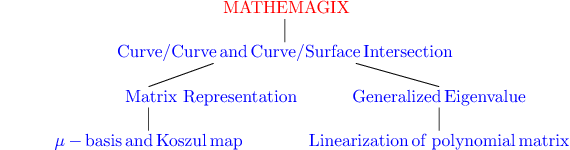
Computing the intersection between algebraic varieties is a
fundamental task in Computer Aided Geometric Design. Several
methods and approaches have been developed for that purpose.
Some of them are based on matrix representations of the
objects that allow to transform the computation of the
intersection locus into generalized eigencomputations . The
aim of our works is to compute the matrix representation of
these objects and to show that similar algorithms can be
implemented even if the matrix representation used are non
square matrices. Notice that recent researches, known under
the name of the moving lines, moving surfaces,  -basis method, have demonstrated that
these non square representation matrices are much easier to
compute than square representation matrices. In particular,
the matrix representation of rational space curves are
always non-square matrices
-basis method, have demonstrated that
these non square representation matrices are much easier to
compute than square representation matrices. In particular,
the matrix representation of rational space curves are
always non-square matrices
The approach to the curve/curve, curve/surface intersection
problem that we develop in our works contain two main parts.
The first one is the computation of a matrix representation
of the curve and surface from theirs parametrization. This
work requires advanced concepts of commutative algebra and
algebraic Geometry such as: Elimination theory, free
resolution of modules, Koszul complex, approximate complex,
Fitting invariant, MacRae invariant, algebraic variety,
primary decomposition of ideal,....One of the most effective
algorithm for computing them is via Grobner basis of
modules, Grobner basis of ideals or via  -basis
of a set polynomial. All of this computings are symbolic
computations.
-basis
of a set polynomial. All of this computings are symbolic
computations.
After combining this matrix representation of the curve and the surface with the parameterization of the curve, the second part consists of a matrix reduction and some eigenvalue computations. In this part, we use the technics of linear algebra such as: Kronecker form of a pencil matrix, Smith form of univariate polynomial matrix, LU-decomposition, QR-decomposition, Sylvester matrix, Bezout matrix,.... As a particularity of our method, these two parts can be performed either by symbolic exact computations or by numerical approached computations. However, it seems that a good combination is to choose a symbolic treatment for the first part, so that the change of representation does not affect the intersection locus, and then using numerical computations, typically LU-decompositions, QR-decomposition and eigenvalues computations, to end the algorithm.
We develop this package in order to solve all problems which we talk above. Hereafter, we introduce some functions for explaining the work which we make.
Mathemagix: http://www.mathemagix.org/www/main/index.en.html
Package: Algebramix (Symbolic Computation).
Packages: Realroot, Numerix, Linalg (Numeric Computation).
2.-basis of
a set polynomials
Given the set of homogeneous polynomial of the same degree
  in
in
 with
with  .
.
 .
.
By Hilbert-Burch Theorem: Syz( )
is free and graded
-module of rank n. Chosing a basis
)
is free and graded
-module of rank n. Chosing a basis
 of
of  .
.
is called a  -basis of
  .
.
 in
in  with n:=max (deg
 and .
Homogenizing
and .
Homogenizing  by new variable t
which are denoted
by new variable t
which are denoted  such that are homogeneous polynomial in K[s,t] of
the same degree n. We chose a basis
of Syz
such that are homogeneous polynomial in K[s,t] of
the same degree n. We chose a basis
of Syz  . Then, the set
  is called a -basis of
the set univariate polynomial
is called a -basis of
the set univariate polynomial .
.
Function: mubase f gives the  -basis of the set
of univariate polynomial
-basis of the set
of univariate polynomial  .
.
Function: mubase_homogeneous (f,var)
gives the -basis
of the set of homegenous polynomial
with homogeneous variable var.
 .
.
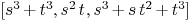
Then -basis of
is
Mmx]
include
"shape/matrixrepresentation/mubase.mmx"
Mmx]
a1:=polynomial(0,0,3);a2:=polynomial(0,3,0,-3);
a3:=polynomial(1,1); a4:=polynomial(1,0,1);
Mmx]
f:=[a1,a2,a3,a4]

Mmx]
mubase f

Mmx]
c1:=polynomial(-33,115/2,-49/2,0,1);
c2:=polynomial(-36,61,-25,0,1);
c3:=polynomial(-8,27/2,-13/2,1);c4:=polynomial(1);
Mmx]
f:=[c1,c2,c3,c4]

Mmx]
mubase f

Mmx]
f0:=QQ['x]<<"x^3+x+1";
f1:=QQ['x]<<"x^4-x+2";f2:=QQ['x]<<"x^6-2*x-1";
Mmx]
f:=[f0,f1,f2]

Mmx]
mubase f

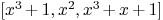
 .
.
Then -basis of
is:
Mmx]
f0:=QQ['x,'y]<<"x^3+x*y^2+y^3";
f1:=QQ['x,'y]<<"x^3-x^2*y";
f2:=QQ['x,'y]<<"x^3+x^2*y+x*y^2";
varf1:=QQ['x,'y]<<"x";
varf2:=QQ['x,'y]<<"y";
Mmx]
f:=[f0,f1,f2]

Mmx]
mubase_homogeneous(f,[varf1,varf2])

3.Matrix representation of parameterized curve and parameterized surface
3.1.Matrix representation of parameterized curve
Let  be
be  homogeneous polynomials in of the
same degree
homogeneous polynomials in of the
same degree  such that
  . Consider the regular map

Algebraic curve  := Image of
  which is called a rational
curve.
which is called a rational
curve.
 with entries in
 is said to be a
representation of a parameterized curve
is said to be a
representation of a parameterized curve  if
if
The rank of
is generically full rank,
drops exactly on
the curve  .
.
Now, we give some example to compute the matrix
representation of a parameterized curve. We focus on curve
in  and
and  because they are the most interesting cases.
Function: matrix_rep_curve_plane_homogeneous(curplane,varcur,varimplcurve).
Function: matrix_rep_curve_plane(curplane,varimplcurve).
Function:
matrix_rep_curve_space_homogeneous(curspace,varcur,varimplcurve).
Function: matrix_rep_curve_space(curspace,varimplcurve).
 .
.
Then a matrix representation of is
Mmx]
include
"shape/matrixrepresentation/curvesurface.mmx"
Mmx]
R:=QQ['s,'t,'x,'y,'z,'w];
Mmx]
curplane:=[R<<"s^3+t^3",R<<"s^2*t",R<<"s^3+s*t^2+t^3"]
Mmx]
varcur:=[R<<"s",R<<"t"]

Mmx]
varimplcurve:=[R<<"x",R<<"y",R<<"z"]

Mmx]
matrix_rep_curve_plane_homogeneous(curplane,varcur,varimplcurve)

Mmx]
curplane:=[polynomial(1,0,0,1),
polynomial(0,0,1),polynomial(1,1,0,1)]
Mmx]
matrix_rep_curve_plane(curplane,varimplcurve)
 .
.
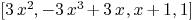
Then a matrix representation of is
Mmx]
curspace:=[R<<"3*s^2*t",R<<"-3*s^3+3*s*t^2",R<<"s*t^2+t^3",R<<"t^3"]

Mmx]
varimplcurspace:=[R<<"x",R<<"y",R<<"z",R<<"w"]

Mmx]
matrix_rep_curve_space_homogeneous(curspace,varcur,varimplcurspace)
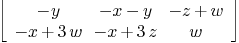

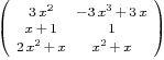
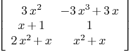
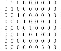
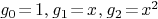
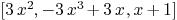
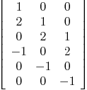
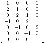
Then a matrix representation of is
Mmx]
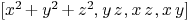
curspace:=[polynomial(0,0,3),polynomial(0,3,0,-3),polynomial(1,1),
polynomial(1)]
Mmx]
matrix_rep_curve_space(curspace,varimplcurspace)
3.2. Matrix representation of parameterized surfaces
Suppose given a parametrization

of a surface  such that
  .
.
with entries in  is said to be a representation of surface
  if
if
The rank of
is generically full rank,
drops exactly on the
surface  .
.
 .
Then a matrix representation of is
.
Then a matrix representation of is
Function: matrix_rep_surface(surface,varsur,varimplsur).
Mmx]
include
"shape/matrixrepresentation/curvesurface.mmx"
Mmx]
R:=QQ['x,'y,'z,'w];
Mmx]
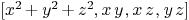
Steine:=[R<<"x^2+y^2+z^2",R<<"x*y",R<<"x*z",R<<"y*z"]
Mmx]
varimplsur:=[R<<"x",R<<"y",R<<"z",R<<"w"]
Mmx]
varsur:=[R<<"x",R<<"y",R<<"z"]
Mmx]
matrix_rep_surface(Steine,varsur,varimplsur)
 :
: .
Then a matrix representation of
.
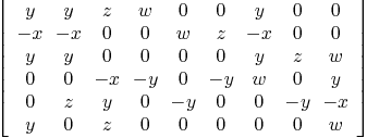
Then a matrix representation of  is
is
Mmx]
Sphere:=[R<<"x^2+y^2+z^2",R<<"2*x*z",R<<"2*x*y",R<<"x^2-y^2-z^2"]

Mmx]
matrix_rep_surface(Sphere,varsur,varimplsur)
Mmx]
4.Polynomial Matrix and Generalized eigenvalues
4.1. Linearization of a polynomial matrix
Let  and
and  be
two matrices of size
be
two matrices of size  . We will call a
generalized eigenvalue of A and B a value in the
set
. We will call a
generalized eigenvalue of A and B a value in the
set

Suppose given an -matrix  with polynomial entries
  .
It can be equivalently written as a polynomial in
.
It can be equivalently written as a polynomial in  with coefficients -matrices
with entries in
with coefficients -matrices
with entries in  : if
: if  then
then

where  .
.
of size  that are given by


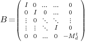
where I stands for the identity matrix and  stand for the transpose of the matrice
  .
.
Function: list_coefficients_matrix M
gives the list of matrices:  .
.
Function: firstcompanionmatrix M gives the matrix A.
Function: secondcompanionmatrix M gives the matrix B.
 .
.
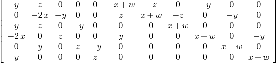
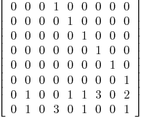
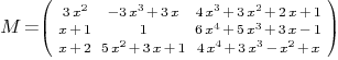
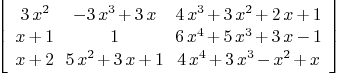
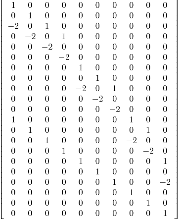
Then  and the generalized companion
matrices of M are
and the generalized companion
matrices of M are
Mmx]
include
"shape/matrixrepresentation/pencilregular.mmx"
Mmx]
M:=matrix(polynomial(0,0,3),polynomial(0,3,0,-3);polynomial(1,1),
polynomial(1);polynomial(0,1,2),
polynomial(0,1,1))
Mmx]
degree M

Mmx]
list_coefficients_matrix M

Mmx]
firstcompanionmatrix M
Mmx]
secondcompanionmatrix M
Mmx]
4.2.Regular matrix and generalized eigenvalues

 is called
to be regular pencil matrices if A',B' are square matrices
and B' is invertible.
is called
to be regular pencil matrices if A',B' are square matrices
and B' is invertible.
Function: pencilregular(A,B) gives (A',B').
Function: generalized_eigenvalues M gives the list of generalized eigenvalues of M(t).
.
Regular pencil matrices (A',B') of M and generalized eigenvalues of M are:
Mmx]
include
"shape/matrixrepresentation/pencilregular.mmx"
Mmx]
M:=matrix(polynomial(0,0,3),polynomial(0,3,0,-3);polynomial(1,1),
polynomial(1); polynomial(0,1,2),
polynomial(0,1,1))
Mmx]
A:=firstcompanionmatrix M
Mmx]
B:=secondcompanionmatrix M
Mmx]
pencilregular(A,B)

Mmx]
generalized_eigenvalues M

Mmx]
 .
.
Then the generalized eigenvalues of M are:
Mmx]
include
"shape/matrixrepresentation/pencilregular.mmx"
Mmx]
M:=matrix(polynomial(0,0,3),polynomial(0,3,0,-3),polynomial(1,2,3,4);
polynomial(1,1),polynomial(1),
polynomial(-1,3,0,5,6); polynomial(2,1),
polynomial(1,3,5), polynomial(0,1,-1,3,4))
Mmx]
generalized_eigenvalues M

Mmx]
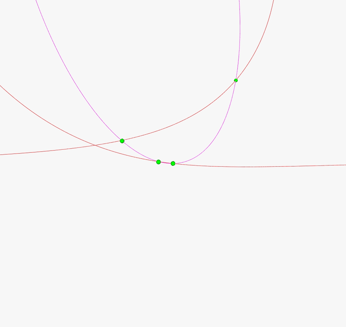
5.Parameterized curve/curve intersection
 |
(1) |
 |
(2) |
 : Representation matrix of
  .
.
Representation matrix of  :
:

As a consequence of the properties of a representation matrix, we have the following easy property.
 , then
 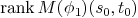 drops
iff the point
drops
iff the point 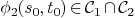 .
.
Hereafter, we give some example which are focussed on the
intersection of the rational curves in the plane  and the intersection of the rational curves in
the space
and the intersection of the rational curves in
the space  .
.
Function: intersection_curve_plane(curve1,curve2).
Function: intersection_curve_space(curve1,curve2).
Function:
intersection_curve_plane_homogeneous(curve1,varcur1,curve2,varcur2).
Function: intersection_curve_space_homogeneous(curve1,varcur1,curve2,varcur2).
 :
: 
 :
: 
 are:
are:
Mmx]
include
"shape/matrixrepresentation/curvesurface.mmx"
Mmx]
curve1:=[polynomial(0,0,3),polynomial(0,3,0,-3),
polynomial(1,1)]
Mmx]
curve2:=[polynomial(1),polynomial(0,1),polynomial(0,0,1)]

Mmx]
intersection_curve_plane(curve1,curve2)

Mmx]
 .
.
 .
.
 .
.


 are:
are:
Mmx]
cur1:=[polynomial(-33,115/2,-49/2,0,1),polynomial(-36,61,-25,0,1),
polynomial(-8,27/2,-13/2,1),polynomial(1)]
Mmx]
cur2:=[polynomial(-3,17/2,-11/2,1),polynomial(-6,12,-6,1),polynomial
(-38,125/2,-51/2,0,1),polynomial(1)]

Mmx]
intersection_curve_space(cur1,cur2)

Mmx]

 .
.
are:
Mmx]
include
"shape/matrixrepresentation/curvesurface.mmx"
Mmx]
cur1:=[QQ['x,'y]<<"x^3+3*x^2*y+2*x*y^2+y^3",QQ['x,'y]
<<"x^2*y+2*x*y^2+2*y^3",QQ['x,'y]<<"x*y^2+3*y^3",
QQ['x,'y]<<"y^3"]

Mmx]
cur2:=[QQ['x,'y]<<"x^4-x*y^3+y^4",QQ['x,'y]<<"x*y^3+y^4",QQ['x,'y]<<"x*y^3+2*y^4",QQ['x,'y]<<"y^4"]

Mmx]
varcur:=[QQ['x,'y]<<"x",QQ['x,'y]<<"y"]

Mmx]
intersection_curve_space_homogeneous(cur1,varcur,cur2,varcur)

Mmx]

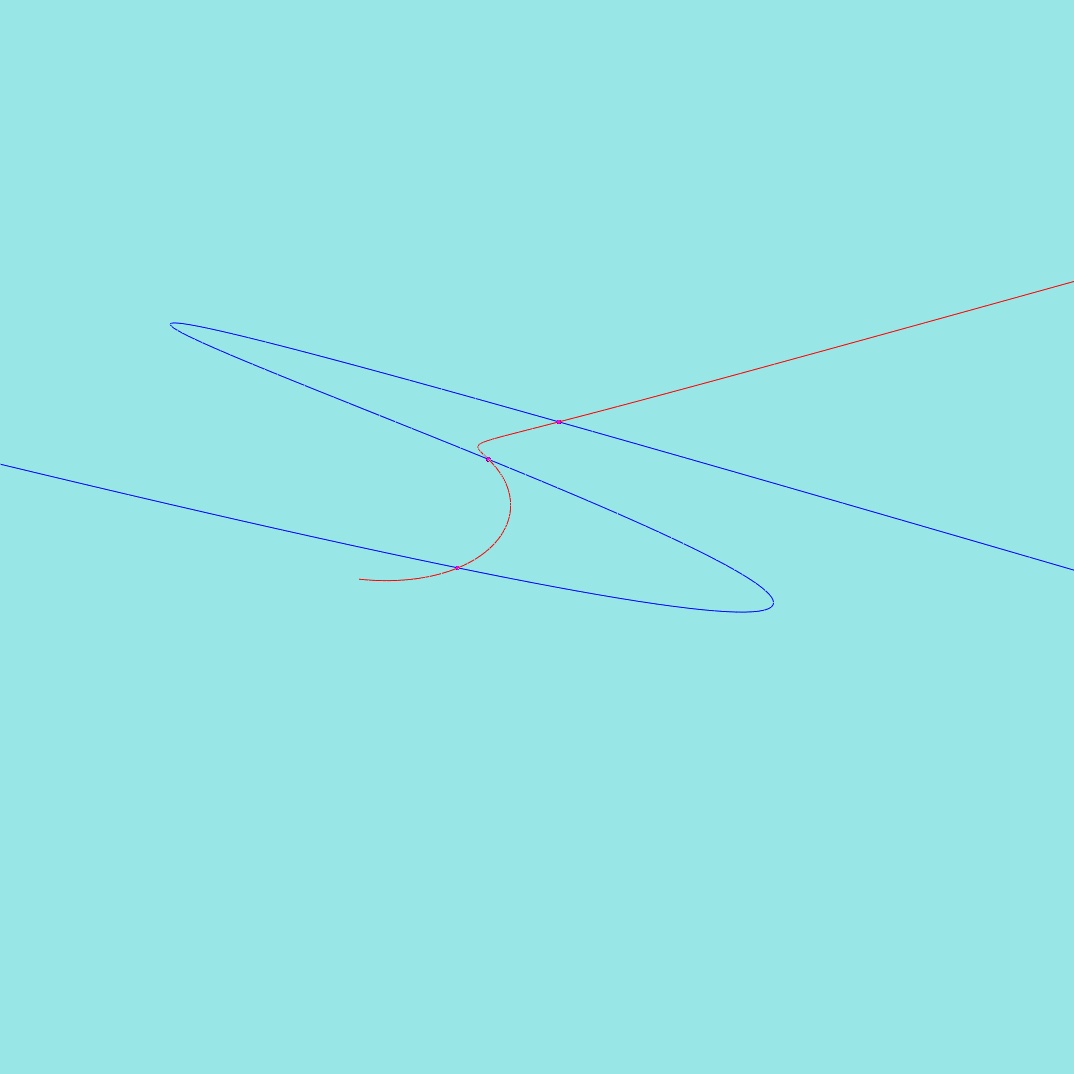
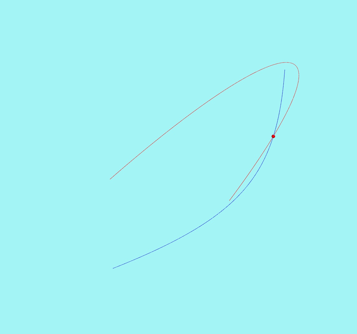
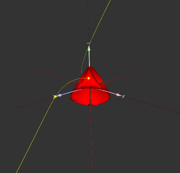
6.Parameterized curve/surface intersection

 .
.
 matrix representation of the surface
 .
.
M(s,t): matrix representation of  :
:

and we have the following easy property:
 , then rank of
  drops iff
  .
.
Function:
intersection_curve_surface_homogeneous(surface,varsur,curve,varcur)
 .
.
Twisted cubic  .
.
 are:
are:
Mmx]
include
"shape/matrixrepresentation/curvesurface.mmx"
Mmx]
R:=QQ['s,'t,'x,'y,'z]

Mmx]
sur:=[R<<"x^2+y^2+z^2",R<<"2*x*z",R<<"2*x*y",R<<"x^2-y^2-z^2"]
Mmx]
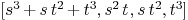
cur:=[R<<"t^3",R<<"s*t^2",R<<"s^2*t",R<<"s^3"]
Mmx]
varsur:=[R<<"x",R<<"y",R<<"z"]
Mmx]
varcur:=[R<<"s",R<<"t"]
Mmx]
intersection_curve_surface_homogeneous(sur,varsur,cur,varcur)

Mmx]
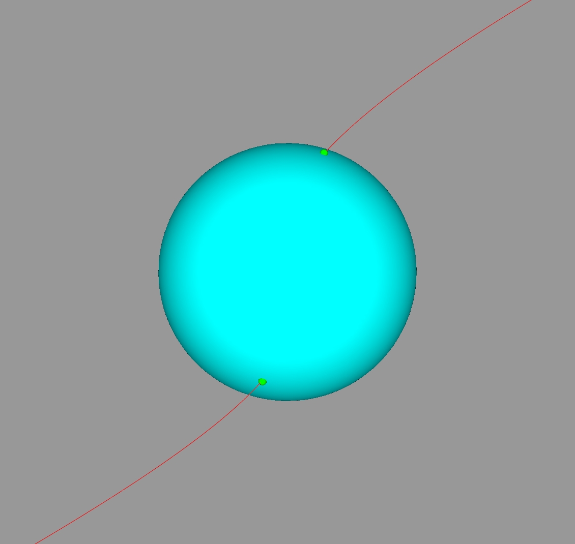

 .
.
Then are:
Mmx]
include
"shape/matrixrepresentation/curvesurface.mmx"
Mmx]
steiner:=[R<<"x^2+y^2+z^2",
R<<"y*z", R<<"x*z",
R<<"x*y"]
Mmx]
varsteiner:=[R<<"x",R<<"y",R<<"z"]
Mmx]
cur:=[R<<"s^3+s*t^2+t^3",R<<"s^2*t",R<<"s*t^2",
R<<"t^3"]
Mmx]
varcur:=[R<<"s", R<<"t"]
Mmx]
intersection_curve_surface_homogeneous(steiner,varsteiner,cur,varcur)

Mmx]
 and (0,0,0).
7. Singular points of parameterized plane curve
Let  be a rational curve of parameterized by the birational
map
be a rational curve of parameterized by the birational
map

 is number of parametervalues
(including multiplicities)
is number of parametervalues
(including multiplicities)  such that
  . Denote
  .
.
Function:
singular_point_plane(curve,varcur,int)
int:=.
 .
.
 of multiplicity 2 and
 of multiplicity 3.
Mmx]
include
"shape/matrixrepresentation/singular_point.mmx"
Mmx]
R:=QQ['t,'x,'y,'z];
Mmx]
curve1:=[R<<"t^5-2*t^3+2",
R<<"t^4+3",
R<<"1"]

Mmx]
varcur:=[R<<"t",R<<"x",R<<"y",R<<"z"];
Mmx]
singular_point_plane(curve1,varcur,2)


Mmx]
singular_point_plane(curve1,varcur,3)

Mmx]
singular_point_plane(curve1,varcur,4)

 .
.
Mmx]
include
"shape/matrixrepresentation/singular_point.mmx"
Mmx]
curve2:=[R<<"t^4-40*t^3+40*t+1",
R<<"t^4+480*t^2+1",
R<<"t^4+40*t^3+480*t^2+40*t+1"]

Mmx]
singular_point_plane(curve2,varcur,2)

Mmx]
singular_point_plane(curve2,varcur,3)
 .
.
Mmx]
include
"shape/matrixrepresentation/singular_point.mmx"
Mmx]
f:=R<<"t";g:=R<<"t+1";h:=R<<"2*t+1";k:=R<<"3*t^2+2*t+1";
Mmx]
curve3:=[f^2*g^6*h^2,f^3*h^2*k,-g^10]

Mmx]
singular_point_plane(curve3,varcur,2)

Mmx]
singular_point_plane(curve3,varcur,3)
Mmx]
singular_point_plane(curve3,varcur,4)

Mmx]
singular_point_plane(curve3,varcur,6)

Mmx]
8.Conclusion
-
Introduce new matrix- based representation of rational space curves and parameterized surfaces.
-
Transfer the solving of the curve/curve, curve/surface intersection problem into the eigenvalues computing problems.
-
Remove the Kronecker bad blocks of the pencil of matrices
 in order to extract the regular pencil
  .
.
-
Illustrate the advantages of matrix representation by addressing several impotant problems: the intersection problems and the computation of singularities of rational curves.
9.Some more funtions
9.1.Solve the equation of univariate polynomial
Let  be univariate
polynomial with the rational coefficients. Funtion solve f is given
to find all roots of equation
be univariate
polynomial with the rational coefficients. Funtion solve f is given
to find all roots of equation  .
.
Mmx]
include
"shape/matrixrepresentation/solvepolynomial.mmx"
Mmx]
f:=QQ['x]<<"x^40+x^3-x^2+x+1"

Mmx]
solve f

Mmx]
g:=polynomial(0,0,1)

Mmx]
solve g^2

9.2.Graded Koszul map
-
Denote by
 the set
homogemeous polynomial of degree k and
the set
homogemeous polynomial of degree k and  then matrix
reperesentation of graded Koszul map (in the
standard basis)
then matrix
reperesentation of graded Koszul map (in the
standard basis)

Function: matrix_multiply_curve(f,var,n,d)
Mmx]
include
"shape/matrixrepresentation/curvesurface.mmx"
Mmx]
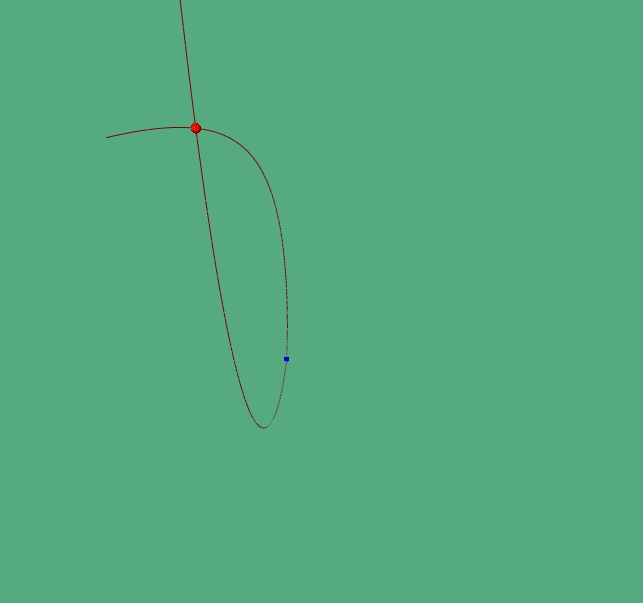
f:=QQ['s,'t]<<"s^3+2*s^2*t-t^3"
Mmx]
degree f
Mmx]
var:=[QQ['s,'t]<<"s",QQ['s,'t]<<"t"]
Mmx]
matrix_multiply_curve(f,var,2,3)
Mmx]
matrix_multiply_curve(f,var,3,3)
-
Denote by
 the set
homogemeous polynomial of degree k and
the set
homogemeous polynomial of degree k and  then matrix
reperesentation of graded Koszul map (in the
standard basis)
then matrix
reperesentation of graded Koszul map (in the
standard basis)

Function: matrix_multiply_surface(f,var,n,d)
Mmx]
f:=QQ['s,'t,'u]<<"s^2-2*t^2+u^2"

Mmx]
degree f

Mmx]
var:=[QQ['s,'t,'u]<<"s",QQ['s,'t,'u]<<"t",QQ['s,'t,'u]<<"u"]

Mmx]
matrix_multiply_surface(f,var,2,2)

Mmx]
matrix_multiply_surface(f,var,3,2)
9.3.Extented Euclidean Algorithm
Given two polynomials  with
with  . It exits two
polynomials of smallest degree
. It exits two
polynomials of smallest degree  such that
  .
.
Function: EEA(f,g) give  .
.
Mmx]
include
"shape/matrixrepresentation/EEA.mmx"
Mmx]
f:=QQ['x]<<"x^3+3*x-4"

Mmx]
g:=QQ['x]<<"x^5-3*x^4+4*x-2"
Mmx]
EEA(f,g)

Mmx]
gcd(f,g)

Mmx]
L:=EEA(f,g)
Mmx]
L[1]*f+L[2]*g

9.4.Another functions
Mmx]
L:=[b1,b2,b3,b4]

Mmx]
delete(L,b1)

Mmx]
delete(L,b4)

Mmx]
delete(L,a)
Mmx]
L:=[b1,b1,b2,b2,b3,b4,b4,b4]

Mmx]
delete_dif L
Mmx]
10.Some future works
-
Using subresultant of
-basis to
solve some problems of rational space curves.
-
Intersection multiplicity problem between two rational curves.
-
Intersection parameterized surface/surface.
-
Singular points of parameterized surfaces.
-
Develop the implementation of the software Mathemagix to solve the above purposes.
11. References
1. N. Song, R. Goldman, -bases
for polynomial systems in one variable, Comput. Aided
Geom. Design 26 (2) (2009) 217–230.
2. T. Luu Ba, L. Busé, B. Mourrain, Curve/surface intersection problem by means of matrix representations, in: SNC '09: Proceedings of the 2009 conference on Symbolic numeric computation, ACM, New York, NY, USA, 2009, pp. 71–78.
3. L. Busé and M. Chardin, Implicitizing rational hypersufaces using approximation complexes. J. Symbolic Comput. 40(4-5): 1150-1168, 2005.
4. L. Busé and T. Luu Ba, Matrix-based implicit representations of rational algebraic curves and applications. To appear Computed Aided Geometric Design 2010.
5. F. Chen, W. Wang and Y. Liu, Computing singular points of plane rational curves. J. Symbolic Comput. 43 , 92-117, 2008.
6. The software Axel (http://axel.inria.fr) and Mathemagix (http://www.mathemagix.org).